All described methods are available in Topoly Python package (or will be soon available).
In mathematical knot theory, knots are defined as any embedding of circle in 3D space. The main difference between the conventional notion of knot and mathematical one is that the latter form loops (i.e. they are closed and do nat have any free ends). Still the mathematical notion of knotting has found applicationss in a study of entanglement of open chains, e.g. proteins. So far four types of knots have been found in proteins, these are: the trefoil knot (31), the number eight knot (41), the 3-twist knot (52) and the Stevedore knot (61) (besides the trivial knot, called also an unknot, 01). This notation is described below.
Every 3D knot comfiguration can be represented as a knot diagram. To obtain a knot diagram, we project it onto a plane (we draw it on a piece of paper) so that the strands intersect transversely and there are never three or more strands crossing at one point in the projection. Then we mark ar each crossing which strand is higher in the direction normal to the projection plane.
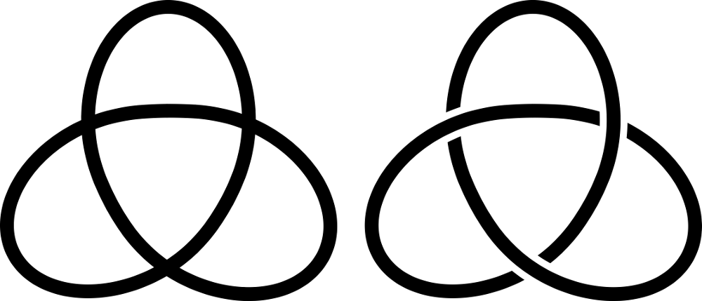
Figure 1. Left: projection of a 31 knot, right: diagram of 31 knot.
Different knot diagrams of the same knot type can have different number of crossings. But every knot have has a diagram with a minimal number of crossings which cannot be further simplified. This representation is called a minimal knot representation and it is a basis for the naming convention for knot types.
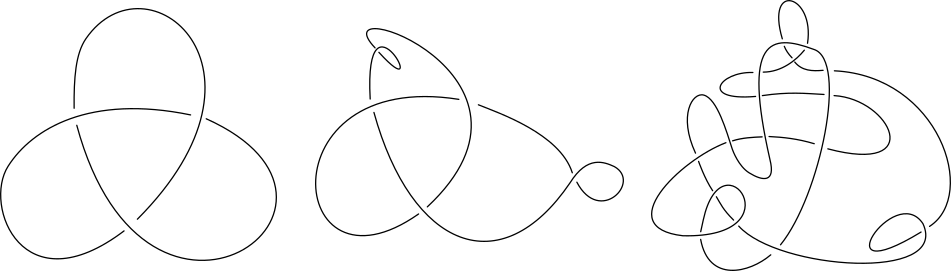
Figure 2. Despite having different number of crossings, both of these diagrams represent a trefoil knot (31 ). The left diagram is a minimal 31 knot representation.
The knot notation is based on a number of crossings in minimal knot representation, with which each name begins. For example the knot 73 has 7 crossings in its minimal representation. The second number (subscript) distinguishes different knot types with the same number of crossings in minimal representation. The 73 knot is the third knot type amongst the list of prime 7-crossing knot types. If a knot can be divided into two simpler, but non-trivial, knots, it is called a composite knot. For example the composition of knots 31 and 41 is denoted by 31#41. If a knot type is not composite, then it is known as a prime knot type.
Knot theory invariants, which are used to classify knot types, can by applied to closed chains only. In general, proteins are open chains. Therefore if one wants to use knot invariants, the open chain needs to be closed in some fashion. Closing the open chain can be done in a number of ways, which can be divided into deterministic ones and probabilistic ones. In our server three closure options are available:
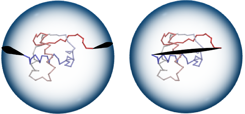
Figure 3. ”Two points” closure method (left): two random points on a large sphere are randomly chosen and connected by line segments to the endpoints of a chain, and to each other by an (auxiliary) arc. ”Direct” closure method (right): chain end-points are connected by a straight line segment. Image from KnotProt database.
HOMFLY-PT, one of most general and best discriminating knot polynomial, is a polynomial of two variables, usually denoted as m and l, and has the ability to recognize chirality of knots, as well as disjointed unions of knots and links, in many cases. It can by computed using recursive skein relation on knot diagram via:

where L+ , L- and L0 are diagrams of knots/links that differ just in the region near one crossing as is presented in the Figure below. Unfortunetely, this results in expotential time-complexity of computation as a function of the number of crossings.
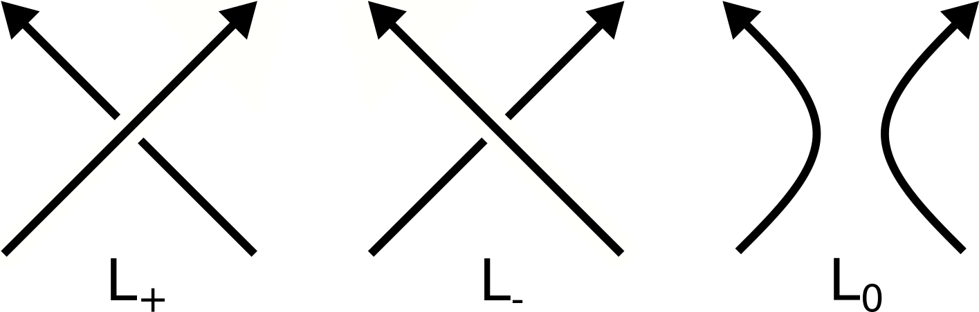
Figure 4. Crossings L+, L-, L0. During computation of a knot polynomial using the skein relation above, some crossings from a knot diagram are transformed into other types to create simpler diagrams, eventually ending in a union of trivial knots. Then these simpler diagrams are used to compute knot polynomial of the original diagram. The HOMFLY-PT polynomial of a trivial knot (an unknot, a circle) is 1. HOMFLY-PT polynomials for examples of knots are presented in the Table 1.
Table 1. Examples of HOMFLY-PT polynomials and Alexander polynomials for a few knot types.
| Knot type | 01 | 31 | 41 | 51 | 52 | 61 |
 unknotted |
 trefoil knot |
 figure-8 knot |
 cinquefoil knot |
 three-twist knot |
 Stevedore knot |
|
| Values of HOMFLY-PT polynomial | P(01) = 1 | P(+31) =- l-4 - 2l-2 + l-2m2 | P(41 )=- 1 - l-2 - l2 + m2 | P(+51)= 2l-6 - l-6m2 + 3l-4 - 4l-4m2 + l-4m4 | P(+52)= l-6 + l-4 - l-4m2 - l-2 + l-2m2 | P(+61)= l-4 + l-2 - l-2m2 - l2 + m2 |
| P(-31 )=- 2l2 + l2m2 - l4 | P(-51)= 3l4 - 4l4m2 + l4m4 + 2l6 - l6m2 | P(-52 )=- l2 + l2m2 + l4 - l4m2 + l6 | P(-61)= - l-2 + l2 - l2m2 + l4 + m2 | |||
| Values of Alexander polynomial | Δ(01) = 1 | Δ(31) = 1 - t + t2 | Δ(41) = -1 + 3t - t2 | Δ(51) = 1 - t + t2 - t3 + t4 | Δ(52) = 2 - 3t + 2t2 | Δ(61) = -2 + 5t - 2t2 |
The Alexander polynomial was the first polynomial knot invariant. Because it is quite simple, it cannot distinguish chirality of knots, and is always equal to 0 when there exists a disjointed sum of knots. However, the Alexander polynomial is faster to compute then other popular polynomials (it can be done in polynomial time). Conway showed that Alexander polynomial can be computed using the following skein relation:

Alexander polynomial of a trivial knot (an unknot, a circle) is 1. Table 1 shows Alexander polynomials for some example knot types.
For proteins cataloged in our database the process depends on the predicting model category: AlphaFold (AF4 and AF1) or ESM (ESM1). In the case of AlphaFold models (both AF1 and AF4) we use structures that are available for download from the AlphaFold database. However, we only take into account AlphaFold models predictions with prediction score (pLDDT value) of at least 70. You can download a full list of structures that were ignored due to their low pLDDT score from here On the hand, since the ESM Metagenomic Atlas does not contain structures based on the sequences from Uniprot and thus equivalent to the AlphaFold models, we generate those 3D models using the ESM fold v1 model available on the ESM Github repository.
The full structure (processed either by the server or cataloged) is first checked using the HOMFLY-PT polynomial. We recognize knots which have at most 12 crossings in their minimal representation. In our initial study of the whole AlphaFold dataset of 200MM structures we first used probabilistic closing with 200 random closures and later verified those structures that were identified as potentially knotted with a higher number of 500 closures. If we find a non-trivial knot, then the structure is further processed and the knot core is determined. In the case of AlphaFold v1 we also calculated whole knot maps, however, for AF4 and ESM1 we decided not to compute those due to the large scale of computing power that would be necessary for this task. On the other hand, users can run a knot map calculation for any structure through our web server. Because of that the knot core identification was also done differently: for AF1 we used an algorithm that analyzed the knot maps and determined both the knot fingerprints and the knot cores of all knot types formed by the structure. For AF4 and ESM1 we used our heuristic algorithm to determine the knotcore of the knot identified for the full chain only - the same algorithm is used in the web server when the user chooses not to run a full knot map calculation.
By "finding a knot using probabilistic closure" we mean that the dominant knot type is non-trivial with a probability at least 42% and the probability for an unknot is smaller than 50%. When computing a knot map, the faster Alexander polynomial is used.
You can download a full list of structures found to be unknotted from here
All methods described here are available in Topoly Python package (or will be soon available).
Due to the scale of the computations necessary appropriate distributed computing tools had to be developed to coordinate the computing process for all the structures in the database. The kafka-slurm-agent was developed by Paweł Rubach for this task. Thanks to this tool it was possible to combine the power of 3 independent slurm managed Linux clusters as well as a number of individual workstations to run this knot identification process on 200MM structures. Only the first phase of the knot identification on AlphaFold v4 models involved using a total of 70 nodes, with around 2000 cores and processing of 23 TiB of data.